At its core, the idea of probability is very unintuitive. When I say something like, “there is more than a 50% chance of rain tomorrow” or “the chance of me flipping heads on a fair coin is 50%”, I’m alluding to varying notions of probability, and both these statements carry very different meanings.
Different Ways of Thinking
Mostly, when people get introduced to the idea of probability, it is done through this idea of trying to quantify the chance of some event happening given all possible outcomes. But, it is very hard to reason about some situations with this “possible outcomes” framing in mind.
For instance, take an example where I say something like, “Candidate B has a 60% chance of winning the election.” In this case, it is unclear what this 60% means in terms of all the possible outcomes. There isn’t necessarily a simple set of equally likely outcomes that we’re counting to get 60%. Instead, in this case, we are using probability to represent/quantify/measure uncertainty about an event, in this case the chance of candidate B winning the election.
The “possible outcomes” framing is one way of constructing probabilities, but probability more generally provides a mathematical framework to reason about uncertainty. But, admittedly, this is a very vague statement about probability. What does it mean to quantify uncertainty? It is unclear how we should interpret the meaning of probabilities.
These are all very simplified explanations of a very rich philosophical question about probability, and if you are interested in learning more, you should read the SEP Page on different interpretations of probability
Objective Interpretation
One way we can view probability is as a tool that is giving us information about some physical underlying phenomenon associated with an event. One very popular interpretation that falls in this camp is called the frequentist interpretation, where probability is seen as the long-run relative frequency of an event across repeated trials. In this framing, we say that a fair coin has a 50% chance of landing on heads, because as the number of flips becomes larger and larger, the proportion of flips that result in heads approaches 50%.
\[\lim_{n \to \infty} \dfrac{\#\{\text{heads in first n flips}\}}{n} = 1/2\]This has a very physical/objective meaning to it: the probability is associated with the behavior of the underlying process. This frequentist interpretation forms the foundation of many important ideas in statistics.
Another well-known interpretation is the propensity interpretation, which sees probability as a measure of the physical tendency (or disposition) of a system to produce a particular outcome. For example, a fair coin can be thought of as having a physical propensity to land on heads with probability 1/2. This points to probability as a real feature of the actual experiment, and not just the uncertainty about it.
Subjective Interpretation
But the objective interpretation is not the only way people think about probabilities. If you think about the frequentist view, for example, it can’t assign meaning to a one-off event like the election, so some people believe that probability doesn’t necessarily have to do with the physical phenomenon of the event, and it has more to do with the degree of subjective belief based on whatever prior information we have about the event. Since real events are never truly repeated, nor truly identical, this way of thinking provides a more natural view of probability as compared to something like a frequentist interpretation. For example, saying that Candidate B has a 60% probability of winning an election can be understood as saying that, given the available evidence, we assign a probability of 0.6 to the event that Candidate B wins. This interpretation does not require the event to be repeatedly observed; instead, probability provides a mathematical framework for reasoning about uncertainty and updating our beliefs as we receive new information.
Formalizing Probability
In this blog, we are interested in learning more about the mathematical theory of probability and its related ideas. Questions about the interpretation of probability will become clearer as we get into the specifics of the subject, but we first need a common mathematical framework from which we can build our ideas. There are many ways to formalize probability, but the most widely used is Kolmogorov’s axiomatization of probability. 11A formalization is, roughly speaking, the process of taking the intuitive ideas and assumptions surrounding a subject and expressing them within a rigorous mathematical framework. Kolmogorov’s axiomatization gives us precisely such a framework for probability, defining the mathematical objects we work with and the rules that probabilities must satisfy. It is the foundation underlying much of modern probability theory, even if most people encounter its ideas without explicitly learning the axiomatic formulation 22There are also other approaches to formalizing probability, such as Cox’s theorem, which we will not explore in this series for now..
For the Kolmogorov formulation33A few things to note here are that these axioms have very clear roots in measure theory, which is a branch of maths that deals with trying to assign a notion of size to things that are non-intuitive and difficult to understand, like sets and subsets. For a brief primer on measure theory, see Measure Theory Basics, we first start with a sample space $\Omega$, which is the set of all possible outcomes, and an event space $F \subseteq 2^{\Omega}$ that is a collection of events. Then we have a measure $P$, which assigns probability, denoted by $P(E)$, to each $E \in F$. $(\Omega, F, P)$ is called the probability space. And, the axioms state that:
- The probability of an event happening is always non-negative; i.e., $P(E) \ge 0 \hspace{1em} \forall E \in F $
- The probability of the entire sample space is equal to 1; $P(\Omega) = 1$
- For a countable sequence of disjoint events (disjoint in set-theoretic terms, meaning the events have no overlap), $A_1, A_2, \ldots, A_k$, then $P(A_1 \cup A_2 \cup \ldots \cup A_k) = P(A_1) + P(A_2) + \ldots + P(A_k)$
From this, we get a formal way of understanding probability as a kind of function that assigns a value between 0 and 1 to events, with the entire sample space having probability 1. Furthermore, for any collection of mutually exclusive (or disjoint) events, the probability of their union is equal to the sum of their individual probabilities. In a simple finite sample space where all outcomes are equally likely, we can calculate the probability of an event as the ratio of the cardinality of the event to the cardinality of the sample space: \(P(A)=\frac{|A|}{|\Omega|}.\)
However, this is only a special case of the more general framework given by the Kolmogorov axioms. The sample space does not need to be finite; it can be infinite, and probability can still be defined on it. In fact, the axiomatic formulation allows us to reason about probability without requiring probabilities to be obtained through counting outcomes at all.
One interesting thing you may have noticed is that nowhere in these axioms do we find the statement which says that probability should be less than or equal to 1. This is actually a result that we can get from using these axioms: if $\Omega$ is the sample space and $A$ is any event that is a subset of $\Omega$ ($A \subset \Omega$) then, we know that since $\Omega = A \cup (\Omega \backslash A)$, using the third axiom, it is pretty clear that $P(A) = 1 - P(\Omega \backslash A)$, and using axiom 1, we can clearly see that: $P(A) \le 1$.
Now, given this formal axiomatic description of probability, we can build on some further results which will be helpful as we move forward. Some of them are listed below, and it will be a good exercise to reason about why they are true:
- If $A \subset B$ then $P(A) \le P(B)$44It’s fairly trivial to see that this is just a more general formulation of the reason that we gave for why $P(A) \le 1$
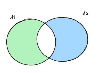
- From the axioms, we know that for a countable sequence of disjoint events, $P(A_1 \cup A_2 \cup \dots \cup A_k) = P(A_1) + P(A_2) + \dots + P(A_k)$, but if they aren’t disjoint, meaning the intersections of these sets aren’t all empty, then the inclusion-exclusion principle holds, meaning for $2$ events: $P(A_1 \cup A_2) = P(A_1) + P(A_2) - P(A_1 \cap A_2)$, for $3$ events: $P(A_1 \cup A_2 \cup A_3) = P(A_1) + P(A_2) + P(A_3) - P(A_1 \cap A_2) - P(A_1 \cap A_3) - P(A_2 \cap A_3) + P(A_1 \cap A_2 \cap A_3)$, and so on for the general case, too.
Now, we will use these ideas to build upon other important ideas of conditioning and independence.
Some More Thoughts
- For the simple case where each outcome is equally likely and there is a finite sample space, the cardinality of those sets will play a very important role in calculating probability. However, counting the number of elements of a set is not always easy. There is a whole field of combinatorics dedicated to doing proper counting, and some basic ideas of permutation and combination will prove very useful when solving probability problems. This guide has some helpful information on that matter.